User Guide

Note: The images in this guide can usually be generated by prefixing the corresponding code example with:

import algoraphics as ag
w, h = 400, 400

and appending this:

c = ag.Canvas(w, h)
c.add(x)
c.png("test.png")

Components

Canvas

The algoraphics library uses the Cartesian coordinate system. This means that while SVG and other computer graphics systems often define the top of the canvas as y=0 with y increasing downward, here y=0 is the bottom of the canvas with y increasing upward. It also means that while the coordinate units are pixels, negative and non-integer values are allowed.

The Canvas object holds a list of objects to be drawn. It has a width, height, and background color (or None for transparent background). It has methods to add one or more objects and clear the canvas (for convenience, new clears the canvas and then adds the objects). The SVG representation of a filled canvas can be retrieved with get_svg, saved to file with svg, or rendered to PNG with png. Likewise, animated graphics can be saved as a GIF with gif.

Shapes

Primitive visible objects are represented with a few Shape subclasses:

Object	Attributes
Circle	c (point), r (float)
Group	members (list), clip (list)
Line	points (list)
Polygon	points (list)
Spline	points (list), smoothing (float), circular (bool)

Shapes can be stored in nested lists without affecting their rendering. The purpose of groups, on the other hand, is to apply things like clipping and shadows to its members. Convenience functions like rectangle exist to define one of these shapes in other ways.

Styles

SVG attributes are used to style shapes and are stored as a dictionary in each shape’s style attribute. Use the set_style function to set one style for one or more shapes, or set_styles to set separate copies of a style to each shape in the list, e.g. to sample from a Color object defined by random parameters.

Parameters

Many algoraphics functions accept abstract parameters that specify a distribution from which to randomly sample.

Algoraphics represents location and other properties declaratively. For example, the end of a tree tranch would be defined relative to the position of its start, and the position of its start would be defined with the same position object as the end of its parent branch.

This makes it simple to animate compound objects in a natural way. In the tree described above, when one branch sways, all of its child branches sway with it.

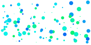
Parameters can also be defined with a distribution. This makes it easy to incorporate subtle or not-so-subtle randomness into the graphics. It also allows basic functions to be used in multiple ways to create different patterns.

For example, a simple command to draw 100 circles can produce this:

w, h = 400, 200
x = 100 * ag.Circle(
    c=(ag.Uniform(10, w - 10), ag.Uniform(10, h - 10)),
    r=ag.Uniform(1, 10),
    fill=ag.Color(hue=ag.Uniform(0.4, 0.6), sat=0.9, li=0.5),
)

or this:

w, h = 400, 200
x = [
    ag.Circle(
        c=(ag.Param([100, 300]), 100),
        r=r,
        fill=ag.Color(hue=0.8, sat=0.9, li=ag.Uniform(0, 1)),
    )
    for r in range(100, 0, -1)
]

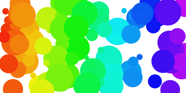
or this:

w, h = 400, 200
x = 100 * ag.Circle(c=(ag.Uniform(0, 400), ag.Uniform(0, h)), r=ag.Uniform(5, 30))
for circle in x:
    color = ag.Color(hue=circle.c.state(0)[0] / 500, sat=0.9, li=0.5)
    ag.set_style(circle, "fill", color)

Parameters can be defined relative to other parameters:

p2y = ag.Delta(start=170, delta=-0.25)
x.append([ag.line((i * 4, 170), (i * 4, p2y)) for i in range(100)])

p2y = ag.Delta(start=100, min=70, max=130, delta=ag.Uniform(-5, 5))
x.append([ag.line((i * 4, 100), (i * 4, p2y)) for i in range(100)])

p2y = ag.Delta(
    start=30,
    min=0,
    max=60,
    delta=ag.Delta(start=0, min=-2, max=2, delta=ag.Uniform(-2, 2)),
)
x.append([ag.line((i * 4, 30), (i * 4, p2y)) for i in range(100)])

ag.set_style(x, 'stroke-width', 2)

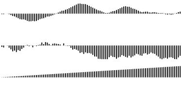
By adding random values to another parameter, you get random-walk-type behavior (middle row of lines above). This chaining doesn’t have to apply directly to the shapes: you can use it to update a parameter representing the change in another parameter, resulting in second-order dynamics (bottom row of lines above).

A parameter can also be defined as a list, from which it will choose the value randomly, or with an arbitrary function, which will be called with no arguments to generate the value.

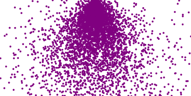
Location Parameters

While Param and its subclasses are used for one-dimensional parameters, two-dimensional, location-based parameters are handled with Point objects:

place = ag.Place(
    ref=(200, 0),
    direction=ag.Normal(90, 30),
    distance=ag.Exponential(mean=50, stdev=100, sigma=3),
)
x = [ag.circle(p, 2, fill="purple") for p in place.values(10000)]

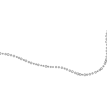
As with single-dimension parameters, Points can be defined relative to others:

x = []
center = (0, 200)
direc = 0
deltadirec = 0
for i in range(300):
    x.append(ag.Circle(center, r=ag.Uniform(2, 4)))
    deltadirec = ag.Clip(deltadirec + ag.Uniform(-5, 5), -10, 10)
    direc = direc + deltadirec
    center = ag.Move(center, direction=direc, distance=ag.Uniform(8, 12))

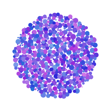
Colors

Colors are represented as objects of the Color class. They are generally defined in the HSL (hue, saturation, lightness) color space. These can be supplied as Param objects:

outline = ag.Circle(c=(200, 200), r=150)
color = ag.Color(
    hue=ag.Uniform(min=0.6, max=0.8), sat=0.7, li=ag.Uniform(min=0.5, max=0.7)
)
x = ex.fill_spots(outline)
ag.set_styles(x, "fill", color)

Shape color attributes like fill and stroke can be set with a string, which will be used as-is in the SVG file. This will work for hex codes, named colors, etc.

Animation

The Dynamic parameter type allows parameters to update at each frame of an animation. For each Dynamic parameter, you define its initial state with a parameter, and then the amount added or multiplied by the previous value to update over time. Every other parameter defined relative to that one is updated too. This allows structures to move in natural ways:

x = []
center = (0, 200)
direc = 0
deltadirec = 0
for i in range(100):
    deltar = ag.Dynamic(0, ag.Uniform(-0.2, 0.2, static=False), min=-0.2, max=0.2)
    r = ag.Dynamic(ag.Uniform(2, 4), delta=deltar, min=2, max=4)
    x.append(ag.Circle(center, r))
    # deltadirec = ag.Clip(deltadirec + ag.Uniform(-5, 5), -10, 10)
    deldeldir = ag.Dynamic(
        ag.Uniform(-5, 5), delta=ag.Uniform(-0.2, 0.2, static=False), min=-5, max=5
    )
    deltadirec = ag.Clip(deltadirec + deldeldir, -10, 10)
    direc = direc + deltadirec
    deltadist = ag.Dynamic(
        ag.Uniform(-2, 2), delta=ag.Uniform(-0.5, 0.5, static=False), min=-2, max=2
    )
    dist = ag.Dynamic(ag.Uniform(8, 12), delta=deltadist, min=8, max=12)
    center = ag.Move(center, direction=direc, distance=dist)
c = ag.Canvas(400, 400)
c.add(x)
c.gif("png/param9.gif", fps=12, seconds=4)

SVG Representation

Shapes are converted to SVG for export. Each type of shape corresponds to a SVG object type or a specific form of one.

algoraphics	SVG
circle	circle
group	g
line	polyline
polygon	polygon
spline	path made of bezier curves

SVG-rendered effects like shadows applied to objects become references to SVG filters, which are defined at the beginning of the SVG file.

By default, the SVG code is optimized using svgo, but this can be skipped for more readable SVG code, e.g. for debugging.

Extras

You can create your own package of reusable functions built upon algoraphics. The extras subpackage is an example of this containing structures, fill functions, and more.

These code snippets are preceded by:

import algoraphics.extras as ex

Images

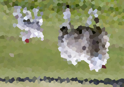
Images can be used as templates for use with patterns or textures. The simplest strategy is to sample colors from the image to color shapes at corresponding locations:

image = ag.open_image("test_images.jpg")
ag.resize_image(image, 800, None)
w, h = image.size
x = ag.tile_canvas(w, h, shape='polygon', tile_size=100)
ag.fill_shapes_from_image(x, image)

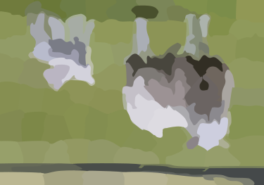
Images can also be segmented into regions that correspond to detected color boundaries with some smoothing, but are constrained to not be too large:

image = ag.open_image("test_images.jpg")
ag.resize_image(image, 800, None)
w, h = image.size
x = ag.image_regions(image, smoothness=3)
for outline in x:
    color = ag.region_color(outline, image)
    ag.set_style(outline, 'fill', color)
ag.add_paper_texture(x)

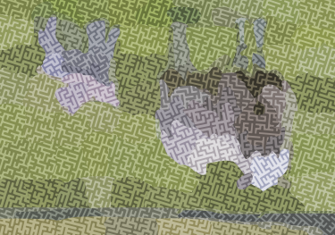
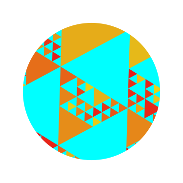
Fill functions can be applied and passed representative colors:

image = ag.open_image("test_images.jpg")
ag.resize_image(image, 800, None)
w, h = image.size
x = ag.image_regions(image, smoothness=3)
for i, outline in enumerate(x):
    color = ag.region_color(outline, image)
    maze = ag.Maze_Style_Pipes(rel_thickness=0.6)
    rot = color.value()[0] * 90
    x[i] = ag.fill_maze(outline, spacing=5, style=maze, rotation=rot)
    ag.set_style(x[i]["members"], "fill", color)
    ag.region_background(x[i], ag.contrasting_lightness(color, light_diff=0.2))

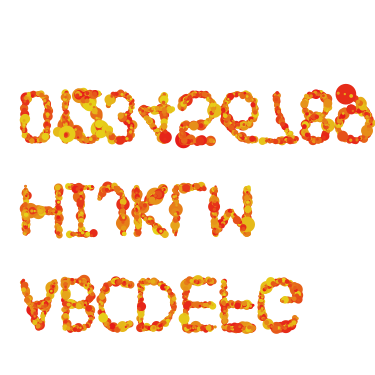
Text

Text can be created and stylized. Characters are generated as nested lists of points (one list per continuous pen stroke) along their form:

color = ag.Color(hue=ag.Uniform(0, 0.15), sat=0.8, li=0.5)

points = ex.text_points("ABCDEFG", 50, pt_spacing=0.5, char_spacing=0.15)
ag.jitter_points(points, 2)
size = ag.Exponential(2.2, stdev=1).values(len(points))
x1 = [ag.circle(c=p, r=size[i], fill=color) for i, p in enumerate(points)]
ag.reposition(x1, (w / 2, h - 50), "center", "top")
c.new(ag.shuffled(x1))

points = ex.text_points("HIJKLM", 50, pt_spacing=0.5, char_spacing=0.15)
ag.jitter_points(points, 2)
size = ag.Exponential(2.2, stdev=1).values(len(points))
x2 = [ag.circle(c=p, r=size[i], fill=color) for i, p in enumerate(points)]
ag.reposition(x2, (w / 2, h - 150), "center", "top")
c.add(ag.shuffled(x2))

points = ex.text_points("0123456789", 50, pt_spacing=0.5, char_spacing=0.15)
ag.jitter_points(points, 2)
size = ag.Exponential(2.2, stdev=1).values(len(points))
x3 = [ag.circle(c=p, r=size[i], fill=color) for i, p in enumerate(points)]
ag.reposition(x3, (w / 2, h - 250), "center", "top")
c.add(ag.shuffled(x3))

x = []

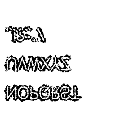
These points can then be manipulated in many ways:

points = ex.text_points("NOPQRST", 40, pt_spacing=0.3, char_spacing=0.15)
ag.jitter_points(points, 8)
size = ag.Exponential(2.2, stdev=1).values(len(points))
x1a = [ag.circle(c=p, r=size[i], fill="black") for i, p in enumerate(points)]

points = ex.text_points("NOPQRST", 40, pt_spacing=1, char_spacing=0.15)
ag.jitter_points(points, 2)
size = ag.Exponential(1.5, stdev=0.5).values(len(points))
x1b = [ag.circle(c=p, r=size[i], fill="white") for i, p in enumerate(points)]

ag.reposition([x1a, x1b], (w / 2, h - 50), "center", "top")
c.new(x1a, x1b)

points = ex.text_points("UVWXYZ", 40, pt_spacing=0.3, char_spacing=0.15)
ag.jitter_points(points, 8)
size = ag.Exponential(2.2, stdev=1).values(len(points))
x2a = [ag.circle(c=p, r=size[i], fill="black") for i, p in enumerate(points)]

points = ex.text_points("UVWXYZ", 40, pt_spacing=1, char_spacing=0.15)
ag.jitter_points(points, 2)
size = ag.Exponential(1.5, stdev=0.5).values(len(points))
x2b = [ag.circle(c=p, r=size[i], fill="white") for i, p in enumerate(points)]

ag.reposition([x2a, x2b], (w / 2, h - 150), "center", "top")
c.add(x2a, x2b)

points = ex.text_points(".,!?:;'\"/", 40, pt_spacing=0.3, char_spacing=0.15)
ag.jitter_points(points, 8)
size = ag.Exponential(2.2, stdev=1).values(len(points))
x3a = [ag.circle(c=p, r=size[i], fill="black") for i, p in enumerate(points)]

points = ex.text_points(".,!?:;'\"/", 40, pt_spacing=1, char_spacing=0.15)
ag.jitter_points(points, 2)
size = ag.Exponential(1.5, stdev=0.5).values(len(points))
x3b = [ag.circle(c=p, r=size[i], fill="white") for i, p in enumerate(points)]

ag.reposition([x3a, x3b], (w / 2, h - 250), "center", "top")
c.add(x3a, x3b)

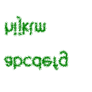
Currently only the characters displayed in these examples are provided, though additional ones can be added on request:

pts = ex.text_points("abcdefg", height=50, pt_spacing=1/4, char_spacing=0.15)
dists = ag.Uniform(0, 10).values(len(pts))
points = [ag.endpoint(p, ag.Uniform(0, 360).value(), dists[i]) for i, p in enumerate (pts)]
radii = 0.5 * np.sqrt(10 - np.array(dists))
x1 = [ag.circle(c=p, r=radii[i]) for i, p in enumerate(points)]
ag.reposition(x1, (w / 2, h - 100), "center", "top")
ag.set_style(x1, "fill", "green")

pts = ex.text_points("hijklm", height=50, pt_spacing=1/4, char_spacing=0.15)
dists = ag.Uniform(0, 10).values(len(pts))
points = [ag.endpoint(p, ag.Uniform(0, 360).value(), dists[i]) for i, p in enumerate(pts)]
radii = 0.5 * np.sqrt(10 - np.array(dists))
x2 = [ag.circle(c=p, r=radii[i]) for i, p in enumerate(points)]
ag.reposition(x2, (w / 2, h - 250), "center", "top")
ag.set_style(x2, "fill", "green")

c.new(x1, x2)

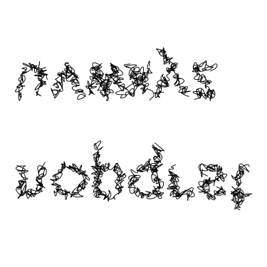
Since generated points are grouped by continuous pen strokes, points within each list can be joined:

strokes = ex.text_points("nopqrst", 60, pt_spacing=1,
                         char_spacing=0.2, grouping='strokes')
for stroke in strokes:
    ag.jitter_points(stroke, 10)
x1 = [ag.spline(points=stroke) for stroke in strokes]
ag.reposition(x1, (w / 2, h - 100), "center", "top")

strokes = ex.text_points("uvwxyz", 60, pt_spacing=1,
                         char_spacing=0.2, grouping='strokes')
for stroke in strokes:
    ag.jitter_points(stroke, 10)
x2 = [ag.spline(points=stroke) for stroke in strokes]
ag.reposition(x2, (w / 2, h - 250), "center", "top")

c.new(x1, x2)

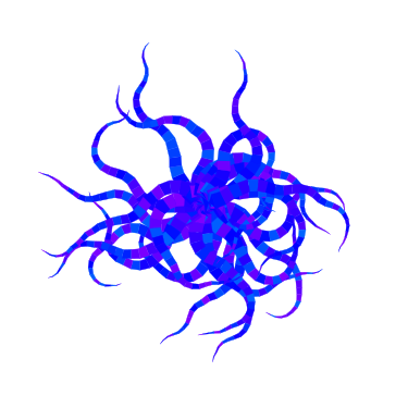
Filaments

Filaments made of quadrilateral segments can be generated:

dirs = [ag.Param(d, delta=ag.Uniform(min=-20, max=20))
        for d in range(360)[::10]]
width = ag.Uniform(min=8, max=12)
length = ag.Uniform(min=8, max=12)
x = [ag.filament(start=(w / 2., h / 2.), direction=d, width=width,
                 seg_length=length, n_segments=20) for d in dirs]
ag.set_style(x, 'fill', ag.Color(hsl=(ag.Uniform(min=0, max=0.15), 1, 0.5)))

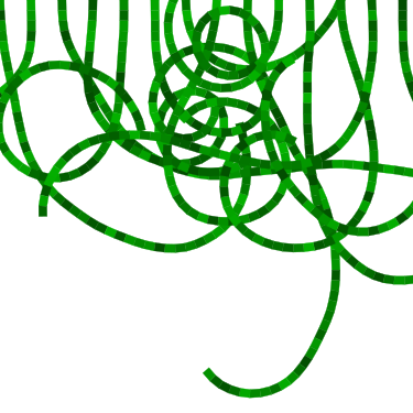
The direction parameter’s delta or ratio attribute allows the filament to move in different directions. Nested deltas produce smooth curves:

direc = ag.Param(90, delta=ag.Param(0, min=-20, max=20,
                                    delta=ag.Uniform(min=-3, max=3)))
x = [ag.filament(start=(z, -10), direction=direc, width=8,
                 seg_length=10, n_segments=50) for z in range(w)[::30]]
ag.set_style(x, 'fill',
             ag.Color(hsl=(0.33, 1, ag.Uniform(min=0.15, max=0.35))))

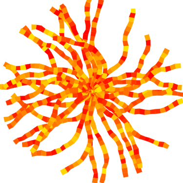
A tentacle is a convenience wrapper for a filament with steadily decreasing segment width and length to come to a point at a specified total length:

dirs = [ag.Param(d, delta=ag.Param(0, min=-20, max=20,
                                   delta=ag.Uniform(min=-30, max=30)))
        for d in range(360)[::10]]
x = [ag.tentacle(start=(w/2, h/2), length=225, direction=d, width=15,
                 seg_length=10) for d in dirs]

ag.set_style(x, 'fill', ag.Color(hsl=(ag.Uniform(min=0.6, max=0.75), 1, 0.5)))

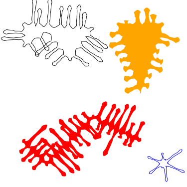
Blow paint

Blow painting effects (i.e., droplets of paint blown outward from an object) can be created for 0D, 1D, and 2D forms:

pts1 = [(50, 50), (50, 100), (100, 70), (150, 130), (200, 60)]
x1 = ag.blow_paint_area(pts1)

pts2 = [(250, 50), (350, 50), (300, 200)]
x2 = ag.blow_paint_area(pts2, spacing=20, length=20, len_dev=0.4, width=8)
ag.set_style(x2, 'fill', 'orange')

pts3 = [(50, 300), (100, 350), (200, 250), (300, 300)]
y = ag.blow_paint_line(pts3, line_width=8, spacing=15, length=30,
                       len_dev=0.4, width=6)
ag.set_style(y, 'fill', 'red')

z = ag.blow_paint_spot((350, 350), length=20)
ag.set_style(z, 'stroke', 'blue')

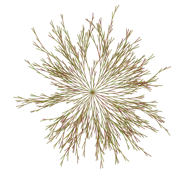
Trees

Trees with randomly bifurcating branches can be generated:

x = [ag.tree((200, 200), direction=d,
             branch_length=ag.Uniform(min=8, max=20),
             theta=ag.Uniform(min=15, max=20),
             p=ag.Param(1, delta=-0.08))
     for d in range(360)[::20]]
ag.set_style(x, 'stroke', ag.Color(hue=ag.Normal(0.12, stdev=0.05),
                                   sat=ag.Uniform(0.4, 0.7),
                                   li=0.3))

Fills

These functions fill a region with structures and patterns.

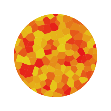
Tiling

These functions divide a region’s area into tiles.

Random polygonal (i.e. Voronoi) tiles can be generated:

outline = ag.circle(c=(200, 200), r=150)
colors = ag.Color(hue=ag.Uniform(min=0, max=0.15), sat=0.8, li=0.5)
x = ag.tile_region(outline, shape='polygon', tile_size=500)
ag.set_style(x['members'], 'fill', colors)

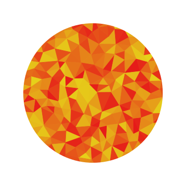
Random triangular (i.e. Delaunay) tiles can be generated:

outline = ag.circle(c=(200, 200), r=150)
colors = ag.Color(hue=ag.Uniform(min=0, max=0.15), sat=0.8, li=0.5)
x = ag.tile_region(outline, shape='triangle', tile_size=500)
ag.set_style(x['members'], 'fill', colors)

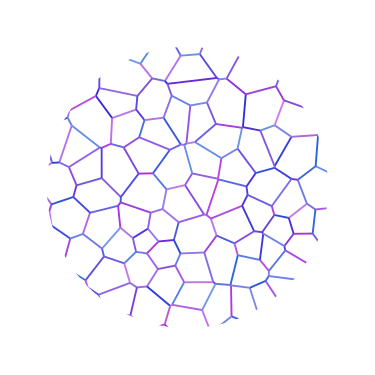
The edges between polygonal or triangular tiles can be created instead:

outline = ag.circle(c=(200, 200), r=150)
colors = ag.Color(hue=ag.Uniform(min=0.6, max=0.8), sat=0.7,
                  li=ag.Uniform(min=0.5, max=0.7))
x = ag.tile_region(outline, shape='polygon', edges=True, tile_size=1000)
ag.set_style(x['members'], 'stroke', colors)
ag.set_style(x['members'], 'stroke-width', 2)

Nested equilateral triangles can be created, with the level of nesting random but specifiable:

outline = ag.circle(c=(200, 200), r=150)
color = ag.Color(hue=ag.Uniform(min=0, max=0.15), sat=0.8, li=0.5)
x = ag.fill_nested_triangles(outline, min_level=2, max_level=5, color=color)

Mazes

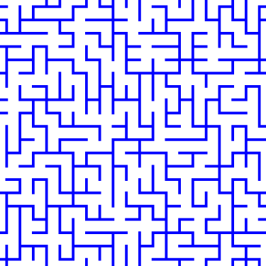
These patterns resemble mazes, but are actually random spanning trees:

outline = ag.rectangle(bounds=(0, 0, w, h))
x = ag.fill_maze(outline, spacing=20,
                 style=ag.Maze_Style_Straight(rel_thickness=0.2))
ag.set_style(x['members'], 'fill', 'blue')

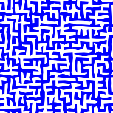
The maze style is defined by an instance of a subclass of Maze_Style:

outline = ag.rectangle(bounds=(0, 0, w, h))
x = ag.fill_maze(outline, spacing=20,
                 style=ag.Maze_Style_Jagged(min_w=0.2, max_w=0.8))
ag.set_style(x['members'], 'fill', 'blue')

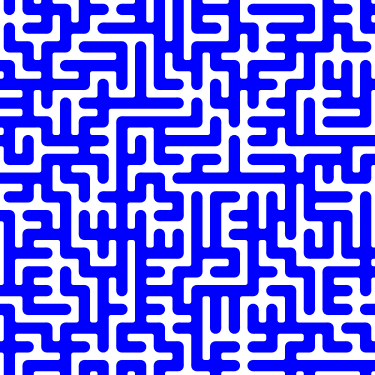
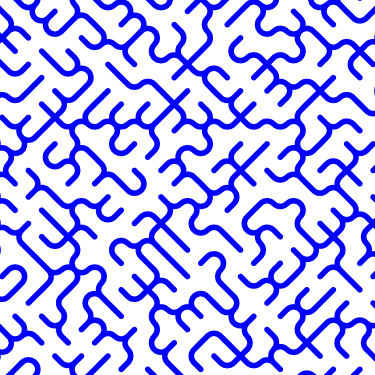
Each style defines the appearance of five maze components that each occupy one grid cell: tip, turn, straight, T, and cross. Each grid cell contains a rotation and/or reflection of one of these components:

outline = ag.rectangle(bounds=(0, 0, w, h))
x = ag.fill_maze(outline, spacing=20,
                 style=ag.Maze_Style_Pipes(rel_thickness=0.6))
ag.set_style(x['members'], 'fill', 'blue')

The grid can be rotated:

outline = ag.rectangle(bounds=(0, 0, w, h))
x = ag.fill_maze(outline, spacing=20,
                 style=ag.Maze_Style_Round(rel_thickness=0.3),
                 rotation=45)
ag.set_style(x['members'], 'fill', 'blue')

Custom styles can be used by creating a new subclass of Maze_Style.

Doodles

Small arbitrary objects, a.k.a. doodles, can be tiled to fill a region, creating a wrapping-paper-type pattern. The ‘footprint’, or shape of grid cells occupied, for each doodle is used to place different doodles in random orientations to fill a grid:

def doodle1_fun():
    d = ag.circle(c=(0.5, 0.5), r=0.45)
    ag.set_style(d, 'fill', 'green')
    return d

def doodle2_fun():
    d = [ag.circle(c=(0.5, 0.5), r=0.45),
         ag.circle(c=(1, 0.5), r=0.45),
         ag.circle(c=(1.5, 0.5), r=0.45)]
    ag.set_style(d, 'fill', 'red')
    return d

def doodle3_fun():
    d = [ag.rectangle(start=(0.2, 1.2), w=2.6, h=0.6),
         ag.rectangle(start=(1.2, 0.2), w=0.6, h=1.6)]
    ag.set_style(d, 'fill', 'blue')
    return d

doodle1 = ag.Doodle(doodle1_fun, footprint=[[True]])
doodle2 = ag.Doodle(doodle2_fun, footprint=[[True, True]])
doodle3 = ag.Doodle(doodle3_fun, footprint=[[True, True, True],
                                            [False, True, False]])
doodles = [doodle1, doodle2, doodle3]
outline = ag.circle(c=(200, 200), r=180)
x = ag.fill_wrapping_paper(outline, 30, doodles, rotate=True)

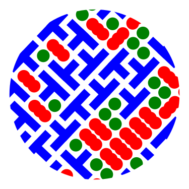
Each doodle is defined by creating a Doodle object that specifies a generating function and footprint. This allows each doodle to vary in appearance as long as it roughly conforms to the footprint.

Other fills

Ripples can fill the canvas while avoiding specified points:

circ = ag.points_on_arc(center=(200, 200), radius=100, theta_start=0,
                        theta_end=360, spacing=10)
x = ag.ripple_canvas(w, h, spacing=10, existing_pts=circ)

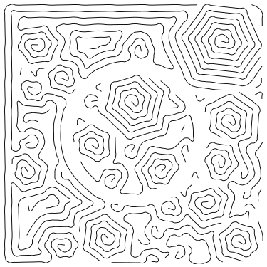
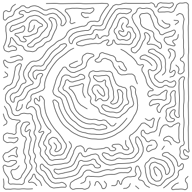
They are generated by a Markov chain telling them when to follow a boundary on the left, on the right, or to change direction. The transition probabilities for the Markov chain can be specified to alter the appearance:

trans_probs = dict(S=dict(X=1),
                   R=dict(R=0.9, L=0.05, X=0.05),
                   L=dict(L=0.9, R=0.05, X=0.05),
                   X=dict(R=0.5, L=0.5))
circ = ag.points_on_arc(center=(200, 200), radius=100, theta_start=0,
                        theta_end=360, spacing=10)
x = ag.ripple_canvas(w, h, spacing=10, trans_probs=trans_probs,
                     existing_pts=circ)

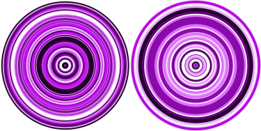
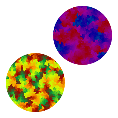
A billowing texture is produced by generating a random spanning tree across a grid of pixels, and then moving through the tree and coloring them with a cyclical color gradient:

outline = ag.circle(c=(120, 120), r=100)
colors = [(0, 1, 0.3), (0.1, 1, 0.5), (0.2, 1, 0.5), (0.4, 1, 0.3)]
x = ag.billow_region(outline, colors, scale=200, gradient_mode='rgb')

outline = ag.circle(c=(280, 280), r=100)
colors = [(0, 1, 0.3), (0.6, 1, 0.3)]
y = ag.billow_region(outline, colors, scale=400, gradient_mode='hsv')

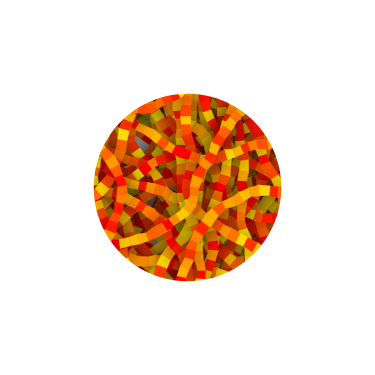
A region can be filled with structures such as filaments using a generic function that generates random instances of the structure and places them until the region is filled:

def filament_fill(bounds):
    c = ((bounds[0] + bounds[2]) / 2, (bounds[1] + bounds[3]) / 2)
    r = ag.distance(c, (bounds[2], bounds[3]))
    start = ag.rand_point_on_circle(c, r)
    dir_start = ag.direction_to(start, c)
    filament = ag.filament(
        start=start,
        direction=ag.Delta(dir_start, delta=ag.Uniform(min=-20, max=20)),
        width=ag.Uniform(min=8, max=12),
        seg_length=ag.Uniform(min=8, max=12),
        n_segments=int(2.2 * r / 10),
    )
    color = ag.Color(hsl=(ag.Uniform(min=0, max=0.15), 1, 0.5))
    ag.set_style(filament, "fill", color)
    return filament


outline = ag.circle(c=(200, 200), r=100)
x = ag.fill_region(outline, filament_fill)
ag.add_shadows(x["members"])

Effects

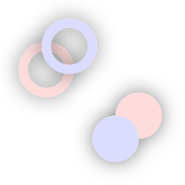
Shadows can be added to shapes or collections, and shapes can be given rough paper textures:

x = [
    ag.circle(c=(100, 150), r=50, stroke="#FFDDDD"),
    ag.circle(c=(150, 100), r=50, stroke="#DDDDFF"),
]
ag.set_style(x, "stroke-width", 10)
ag.add_shadows(x, stdev=20, darkness=0.5)

y = [[
    ag.circle(c=(300, 250), r=50, fill="#FFDDDD"),
    ag.circle(c=(250, 300), r=50, fill="#DDDDFF"),
]]
ag.add_paper_texture(y)

ag.add_shadows(y, stdev=20, darkness=0.5)